Synthetic Natural Gas
www.SyntheticNaturalGas.com

Biomass Gasification  *  Engineering  *  Gas Liquefaction  *  Natural Gas To Liquid  *  Stranded Gas

Synthesis Gas  *  Synthetic Diesel  *  Vacuum Swing Adsorption  *  Waste to Fuel

What is Synthetic Natural Gas?

Synthetic Natural Gas, also referred to as "SNG" and "Substitute Natural Gas," is a green renewable fuel in a gas that contains hydrogen (h2) and carbon monoxide (CO).

According to the Department of Energy, Synthetic Natural Gas (SNG) is one of the commodities that can be produced from coal-derived syngas through the methanation process. 

The economic viability of producing Synthetic Natural Gas through coal gasification is heavily dependent on the market prices of natural gas and the coal feedstock to be used, the value of by-products such as carbon dioxide (CO2) (which could be used for Enhanced Oil Recovery), and additionally the capital cost of the gasification plant. 

Currently, there is only one coal-to-SNG plant currently in commercial operation worldwide. In the middle years of the previous decade, when natural gas prices spiked at previously un-encountered high levels, many proposals were made for new coal-to-SNG plants in the United States. 

In 2010, ten were still proposed or in various stages of development. As natural gas prices have fallen to low levels in the last few years, many or all of these proposed SNG projects as originally envisioned may not move forward to implementation.

marketing@SyntheticNaturalGas.com

Clean Power Generation Systems

CHP Systems (Cogeneration and Trigeneration) Plants 
Have Very  High Efficiencies, Low Fuel Costs & Low Emissions

The CHP System below is Rated at 900 kW and Features:
(2) Natural Gas Engines @ 450 kW each on one Skid with Optional 
Selective Catalytic Reduction system that removes Nitrogen Oxides to "non-detect."

The Effective Heat Rate of the CHP System below is 
4100 btu/kW with a Net System Efficiency of 92%.

Our CHP Systems may be the best solution for your company's economic and environmental sustainability as we "upgrade" natural gas to clean power with our clean power generation solutions. 

Our Emissions Abatement solutions reduce Nitrogen Oxides to "non-detect" which means our CHP Systems can be installed and operated in most EPA non-attainment regions!

Our CHP Systems - (operating in either natural gas fueled cogeneration or trigeneration --- or --- solar cogeneration or solar trigeneration configuration) may be the optimum power and energy solution for customers wanting increased power reliability and decreased energy and environmental costs. A few of the clients and markets that may benefit from our CHP Systems include the following:

• Airports

• Casinos

• Central Plants

• Colleges & Universities

• Dairies

• Data Centers 

• District Heating & Cooling plants

• Food Processing Plants

• Golf/Country Clubs

• Government Buildings and Facilities 

• Grocery Stores

• Hospitals 

• Hotels

• Manufacturing Plants

• Military Bases

• Nursing Homes 

• Office Buildings / Campuses

• Radio Stations

• Refrigerated Warehouses 

• Resorts 

• Restaurants 

• Schools

• Server Farms

• Shopping centers 

• Supermarkets 

• Television Stations

• Theatres

What is Syngas Cleanup?

The synthesis gas (syngas) produced from biomass gasification and plasma gasification plants contains a wide and varying number of pollutants and contaminants before the synthesis gas can be used as a "fuel gas." These pollutants and contaminants may include;

• ammonia

• chlorides

• fine particulates

• heavy metals (trace amounts)

• mercury

• sulfur

To meet environmental emission regulations, as well as to protect downstream processes, the owner/operator of biomass gasification and plasma gasification plants must insure these are removed in a "syngas cleanup" process.

Depending on the application, the synthesis gas may also require "conditioning" to adjust the hydrogen-to-carbon monoxide (H2-to-CO) ratio to meet downstream process requirements.

In applications where very low sulfur (<10 ppmv) synthesis gas is required, converting the carbonyl sulfide (COS) to hydrogen sulfide (H2S) before sulfur removal may also be required.

Typical syngas cleanup and conditioning processes include;

• acid gas removal (AGR) for extracting sulfur-bearing gases and CO2 removal.

• ammonia and chlorides

• catalytic hydrolysis for converting COS to H2S

• cyclone and filters for bulk particulates removal

• solid absorbents for mercury and trace heavy metal removal

• water gas shift (WGS) for H2-to-CO ratio adjustment

• wet scrubbing to remove fine particulates

Introduction to Electricity Generation via Biomass Gasification
The following article adapted from the DOE

Introduction

The U.S. economy uses biomass-based materials as a source of energy in many ways. Wood and agricultural residues are burned as a fuel for cogeneration of steam and electricity in the industrial sector. Biomass is used for power generation in the electricity sector and for space heating in residential and commercial buildings. Biomass can be converted to a liquid form for use as a transportation fuel, and research is being conducted on the production of fuels and chemicals from biomass. Biomass materials can also be used directly in the manufacture of a variety of products.

In the electricity sector, biomass is used for power generation. The Energy Information Administration (EIA), in its Annual Energy Outlook 2002 (AEO2002) reference case,¹ projects that biomass will generate 15.3 billion kilowatthours of electricity, or 0.3 percent of the projected 5,476 billion kilowatthours of total generation, in 2020. In scenarios that reflect the impact of a 20-percent renewable portfolio standard (RPS)² and in scenarios that assume carbon dioxide emission reduction require- ments based on the Kyoto Protocol,³ electricity generation from biomass is projected to increase substantially. Therefore, it is critical to evaluate the practical limits and challenges faced by the U.S. biomass industry. This paper examines the range of costs, resource availability, regional variations, and other issues pertaining to biomass use for electricity generation. The methodology by which the National Energy Modeling System (NEMS) accounts for various types of biomass is discussed, and the underlying assumptions are explained.

A major challenge in forecasting biomass energy growth is estimating resource potential. EIA has compiled available biomass resource estimates from Oak Ridge National Laboratory (ORNL),⁴ Antares Group, Inc.,⁵ and the U.S. Department of Agriculture (USDA).⁶ This paper discusses how these data are used for forecasting purposes and the implications of the resulting forecasts, focusing on biomass used in grid-connected electricity generation applications.

Background

Biomass has played a relatively small role in terms of the overall U.S. energy picture, supplying 3.2 quadrillion Btu of energy out of a total of 98.5 quadrillion Btu in 2000.⁷ The vast majority of it is used in the pulp and paper industries, where residues from production processes are combusted to produce steam and electricity. The industrial cogeneration sector consumed almost 2.0 quadrillion Btu of biomass in 2000. Outside the pulp and paper industries, only a small amount of biomass is used to produce electricity. There are power plants that combust biomass exclusively to generate electricity and facilities that mix biomass with coal (biomass co-firing plants). The electricity generation sector (excluding cogeneration) consumed about 0.7 quadrillion Btu of biomass in 2000. The remaining 0.5 quadrillion Btu of biomass was consumed in the residential and commercial sectors in the form of wood consumption for heating buildings. To put these numbers in perspective, the electricity generation sector consumed 20.5 quadrillion Btu of coal and 6.5 quadrillion Btu of natural gas in 2000.⁸

Biomass played a significant role among renewables in 2000, however, providing 48 percent of the energy coming from all renewable sources. In EIA’s AEO2002 reference case projection, growth in demand for biomass is expected to be modest. In the AEO2002 high renewables case projection, the demand for biomass is higher than in the reference case due to assumptions of reduced initial capital cost⁹ and increased supply. In aggressive RPS cases,¹⁰ the demand for biomass is much higher than projected even in the high renewables case.

Among many reasons for increased biomass utilization in those cases, environmental benefits are the most important. Compared with coal, biomass feedstocks have lower levels of sulfur or sulfur compounds.¹¹ Therefore, substitution of biomass for coal in power plants has the effect of reducing sulfur dioxide (SO₂) emissions. Demonstration tests have shown that biomass co-firing with coal¹² can also lead to lower nitrogen oxide (NO_x) emissions. Perhaps the most significant environmental benefit of biomass, however, is a potential reduction in carbon dioxide (CO₂) emissions.

A closed-loop process is defined as a process in which power is generated using feedstocks that are grown specifically for the purpose of energy production. Many varieties of energy crops are being considered, including hybrid willow, switchgrass, and hybrid poplar. If biomass is utilized in a closed-loop process, the entire process (planting, harvesting, transportation, and conversion to electricity) can be considered to be a small but positive net emitter of CO₂. It is not precisely a net zero emission process in a life-cycle sense, because there are CO₂ emissions associated with the harvesting, transportation, and feed preparation operations (such as moisture reduction, size reduction, and removal of impurities). However, those emissions are not the result of combustion of biomass but result instead from fuel consumption (mostly petroleum and natural gas) for harvesting, transportation, and feed preparation operations.

Although biomass-based generation is assumed to yield no net emissions of CO₂ because of the sequestration of biomass during the planting cycle, there are environmental impacts. Wood contains sulfur and nitrogen, which yield SO₂ and NO_x in the combustion process. However, the rate of emissions is significantly lower than that of coal-based generation. For example, per kilowatthour generated, biomass integrated gasification combined-cycle (BIGCC) generating plants can significantly reduce particulate emissions (by a factor of 4.5) in comparison with coal-based electricity generation processes.¹³ NO_x emissions can be reduced by a factor of about 6 for dedicated BIGCC plants compared with average pulverized coal-fired plants.¹⁴

Biomass Technologies for Electricity Generation

Both dedicated biomass and biomass co-firing are used in the electricity generation sector. New dedicated biomass capacity is represented in NEMS as BIGCC technology. It is assumed that hot gas filtration will be used for gas cleanup purposes in this technology. Hot gas cleanup technology is relatively new, and the U.S. Department of Energy (DOE) and many industrial partners are conducting tests to demonstrate the technology. The alternative to hot gas cleaning is low-temperature gas cleaning. In low-temperature cleaning the gas is quenched with water, and particulates are removed in a series of cyclone vessels. There are advantages and disadvantages associated with both processes.

The advantages of cold gas cleaning are that it is commercially available, the capital cost is relatively low, and the systems are easier to operate than hot gas cleanup systems. The disadvantages of cold gas cleanup are that the cooling process, the cold gas cleanup system, and fuel gas recompression systems reduce the overall process efficiency by up to 10 percent. The gas turbines downstream of the gasifier require the gas at high temperatures and pressure, and therefore the gas that has just undergone cooling for cleanup purposes must be repressurized and reheated in order to conform to gas turbine inlet specifications. The advantages of the newer hot gas cleanup technology are that it allows the process to be operated at higher efficiencies and it generates less waste water than the cold gas cleanup processes. The disadvantages of the hot gas cleanup technology are that operational experience is limited, it has higher costs, and it adds complexity to the process; however, it is considered to be the technologically more advanced choice for new dedicated biomass plants.

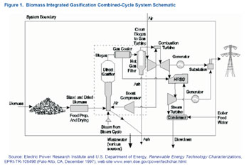
The McNeil Generating Station demonstration project in Burlington, Vermont, is an example of a biomass gasification plant. It has a capacity of 50 megawatts and supplies electricity to the residents of the City of Burlington. This is an existing wood combustion facility whose feedstock is waste wood from nearby forestry operations, including forest thinnings and discarded wood pallets. To this existing wood combustion facility a low-pressure wood gasifier has been added that is capable of converting 200 tons per day of wood chips into fuel gas. The fuel gas, fed directly into the existing boiler (Figure 1) augments the McNeil Station’s capacity by an additional 12 megawatts. The system was designed and constructed in 1998 and attained fully operational status in August 2000.

In addition to the Vermont project, DOE has funded five new advanced biomass gasification research and development projects beginning in 2001. A company in Salt Lake City, Utah, will test new IGCC and integrated gasification and fuel cell (IGFC) concepts based on a new gasifier that uses segregated municipal solid waste, animal waste, and agricultural residues. A company in Minnesota, has begun a project on an atmospheric gasifier with gas turbine at a malting facility, using barley residues and corn stover. A company in Iowa is developing a new combined-cycle concept that involves a fluidized-bed pyrolyzer and uses corn stover as a feedstock. A company in Connecticut, has begun a project that will test a biomass gasifier coupled with an aero-derivative turbine with fuel cell and steam turbine options, using clean wood residues and natural gas as feedstocks. A company in North Carolina, will develop a biomass gasification process that will produce a reburning fuel stream for utility boilers, using clean wood residues. After completion of research and development tests, these projects are candidates for commercialization over the next few years.¹⁵

Biomass co-firing involves combining biomass material with coal in existing coal-fired boilers. Coal-fired boilers can handle a pre-mixed combination of coal and biomass in which the biomass is combined with the coal in the feed lot and fed through an existing coal feed system. Alternatively, boilers can be retrofitted with a separate feed system for the biomass such that the biomass and coal actually mix inside the boiler.

Tacoma Public Utilities is a municipal utility that provides water, electricity, and rail services. Tacoma Steam Plant uses a fluidized bed gasification plant that can co-fire wood, refuse-derived fuel, and coal. The plant runs for only as many hours as necessary to burn the refuse-derived fuel it receives. The City of Tacoma Refuse Utility has modified its resource recovery facility to produce refuse-derived fuel. The generating plant is paid $5.50 per ton to accept the refuse-derived fuel from the Refuse Utility. A memorandum of understanding between the Refuse Utility and Tacoma Public Utilities commits the latter to burn the refuse-derived fuel for electricity generation. Coal is the most expensive fuel for the plant, making it desirable to burn as much biomass as possible.¹⁷ The fuel mix varies from season to season, depending on the availability of biomass feedstocks. The cost of renovating the steam plant to co-fire the biomass fuel was about $45 million. Washington State’s Department of Ecology provided a grant of $15 million to partially offset the renovation costs.

Biomass for electricity generation is treated in four ways in NEMS: (1) new dedicated biomass or biomass gasification, (2) existing and new plants that co-fire biomass with coal, (3) existing plants that combust biomass directly in an open-loop process,¹⁸ and (4) biomass use in industrial cogeneration applications. Existing biomass plants are accounted for using information such as on-line years, efficiencies, heat rates, and retirement dates, obtained through EIA surveys of the electricity generation sector.

Description of Biomass Supply Curves

The biomass fuel price is calculated from regional supply curves, which are an input to the model. The raw data for the supply schedules are available at the State or county level. These are aggregated to form the regional supply schedule by North American Electric Reliability Council (NERC) region. Supply schedules are aggregated for four fuel types: agricultural residues, energy crops, forestry residues, and urban wood waste/mill residues. Table 2 shows the biomass supply available in the United States. The data in Table 2 are based on survey and modeling work by ORNL, the USDA, and Antares Group, Inc. Table 2 represents the maximum supply available in the various regions at a price of $5 per million Btu.¹⁹ A brief description of each type of biomass is provided below:

• Agricultural residues are generated after each harvesting cycle of commodity crops. A portion of the remaining stalks and biomass material left on the ground can be collected and used for energy generation purposes. Residues of wheat straw and corn stover²⁰ are included in the biomass supply schedule used in NEMS. Wheat straw and corn stover make up the majority of crop residues.

• Energy crops are produced solely or primarily for use as feedstocks in energy generation processes. Energy crops includes hybrid poplar,²¹ hybrid willow,²² and switchgrass,²³ grown on cropland acres currently cropped, idled, or in pasture, and in the Conservation Reserve Program (CRP).²⁴

• Forestry residues are the biomass material remaining in forests that have been harvested for timber. Timber harvesting operations do not extract all biomass material, because only timber of certain quality is usable in processing facilities. Therefore, the residual material after a timber harvest is potentially available for energy generation purposes. Forestry residues are composed of logging residues, rough rotten salvageable dead wood, and excess small pole trees.

• Urban wood waste/mill residues are waste woods from manufacturing operations that would otherwise be landfilled. The urban wood waste/mill residue category includes primary mill residues and urban wood such as pallets, construction waste, and demolition debris, which are not otherwise used.

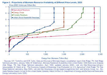
By 2020, the United States is estimated to have a maximum of 7.1 quadrillion Btu of biomass available at prices of $5 per million Btu or lower. Agricultural residues, forestry residues, and urban wood waste/mill residues are currently available. EIA also assumes that energy crops can become available on a commercial basis beginning in 2010. By 2020, the four biomass types are projected to be fairly evenly divided, with agricultural residues providing most of the supply and urban wood waste/mill residues providing the least amount at the high end of the supply curves.

Figure 2 shows the variation in the resource as a function of price. A relatively small portion of the supply is available at $1 per million Btu or less. Feedstock cost is a contributing factor that keeps the growth of biomass-based electricity generation at low levels under AEO2002 reference case conditions. The available low-cost feedstock (<$1 per million Btu) is almost exclusively urban wood waste and mill residues. This category of biomass continues to be the only significant resource available at prices up to about $2 per million Btu. At that price level, agricultural residues become viable as a second source of biomass. Energy crops and forestry residues begin to make significant contributions at prices around $2.30 per million Btu or higher. A brief description of the methodology by which the supply curves are derived is provided below. Table 3 shows the biomass quantities, expressed in various units, that are projected to be available at different price levels.

Agricultural Residue Supply Curve

The underlying assumption behind the agricultural residue supply curve is that after each harvesting cycle of agricultural crops, a portion of the stalks can be collected and used for energy production. Agricultural residues cannot be completely extracted, because some of them have to remain in the soil to maintain soil quality (i.e., for erosion control, carbon content, and long-term productivity). It is assumed that 30 to 40 percent of the residues could be removed from the soil, depending on the State. In terms of acreage, the most important agricultural commodity crops being planted in the United States are listed in Table 4. Corn, wheat, and soybeans represent about 70 percent of total cropland harvested.

The agricultural residue supply curve used in NEMS incorporates only the residues available from corn stover and wheat straws. While this may appear to understate the agricultural residues that are potentially available for energy production, there are compelling reasons for excluding other types of commodity crops. In the case of hay, the whole crop is harvested and fed to livestock; therefore, it is assumed that there would be no useful amount of residue available. An attempt has been made to produce alfalfa, pellet the leaves using adhesive materials, and use the stems as biomass. The processing costs were too high, however, and there was no market for alfalfa pellets in the United States. In the case of tobacco the whole plant is used, leaving little or no residue. Residue from soybeans is relatively small and tends to deteriorate rapidly in the field, making it unsuitable for collection and energy extraction. Barley, oats, rice, and rye are produced in relatively small geographical areas and thus are not likely to have an impact on the national biomass supply curve.

The procedure for estimating the agricultural residue supply curve is as follows. Data on the quantities of corn and wheat produced in each State are available from the USDA.²⁵ From the harvested quantities of corn and wheat grain, a certain amount must be subtracted, representing the amount that the farmer needs to leave on the soil in order to maintain organic matter and prevent erosion. The quantity of residue that must remain depends on the crop type and rotation, soil type, weather conditions, and the tillage system. ORNL is currently preparing detailed estimates of how much residue needs to remain on the soil, taking into consideration these factors. For NEMS, only State-wide average yields and soil carbon needs using a reduced till practice (somewhat similar to mulch till and continuous crop rotations) are being considered.

The price of corn stover and wheat straw includes three components: the cost of collecting the residues, a transportation cost for transporting the material from the farm gate to the energy conversion facility, and a premium paid to farmers to encourage participation. For each harvest operation, a list of needed equipment is determined. Using standard engineering estimates consistent with those used by the USDA, the time per acre required to complete each operation and the cost per hour of using each piece of equipment are calculated.

Both the premiums to farmers and the transportation costs are based on current market practices. Several companies purchase corn stover or wheat straw to produce bedding, insulating materials, particle board, paper, and chemicals. These firms typically pay $10 to $15 per dry ton ($0.58 to $0.87 per million Btu) to farmers to compensate for any lost nutrient or environmental penalties (such as land erosion) that result from harvesting the residues. Studies have shown that transporting giant round bales of switchgrass costs $5 to $15 per dry ton ($0.29 to $0.87 per million Btu) for distances of less than 50 miles. Because agricultural residue bales would be of similar size, weight, and density as switchgrass bales, it is assumed that the cost of transporting bales from the farm gate to the energy conversion facility would be $10 per dry ton ($0.58 per million Btu). It is assumed by ORNL that the premium that would have to be paid to farmers would amount to $10 per dry ton ($0.58 per million Btu), for a total premium and transportation cost of $20 per dry ton ($1.16 per million Btu).

Energy Crop Supply Curve

Energy crops are not currently being commercially grown in the United States. Demonstration programs are underway with DOE funding in Iowa and New York, including IES Utilities Inc.’s biomass co-firing project at its Ottumwa Station plant in Iowa, for which there are plans to produce 200,000 tons of switchgrass harvested from 40,000 to 50,000 acres of land; and NRG’s Dunkirk Station at Dunkirk, New York, where willow from 400 acres of farmland is being co-fired with coal. Therefore, the energy crop supply curve in NEMS represents future resources that could be more profitable at different market prices for farmers to plant in place of existing uses of cropland. An important assumption is that energy crops will not become commercially available until 2010.

The energy crop supply curve prepared by ORNL for EIA has three components: hybrid poplar, hybrid willow, and switchgrass. ORNL uses a model called the Policy Analysis System (POLYSYS) to estimate the quantities of energy crops that could be produced at various prices. POLYSYS is an agricultural sector model that forecasts the production of major agricultural crops. In addition, it has a livestock sector and food, feed, industrial, and export demand functions. POLYSYS was developed and is maintained by the Agricultural Policy Analysis Center at the University of Tennessee and is also used by the USDA Economic Research Service to conduct economic and policy analysis. The underlying assumption in the POLYSYS model is that a farmer will plant and harvest energy crops only if the crop can be sold at a price that assures a profit higher than the profit made by producing conventional agricultural crops on the same piece of land. POLYSYS captures the interaction between energy crops and conventional crops when land is switched from conventional crops to energy crop production. As a joint project between USDA and DOE, POLYSYS has been modified to include dedicated energy crops. POLYSYS uses the 1999 USDA crop and livestock projection as a baseline and can be used to estimate deviations from that baseline.

POLYSYS considers the availability of four types of cropland in the United States: acreage that is currently being planted with traditional crops, idled acreage, acreage in pasture, and acreage in the CRP. The model assumes that energy crop production will be limited to areas that are climatically suited for their production, thus excluding all States in the Rocky Mountain and Western Plains regions. The rationale for these exclusions is that there is a natural rain gradient in the United States, as a result of which land to the west of the gradient generally requires irrigation for crop production, which may have significant environmental penalties. Irrigation has been excluded as a viable management practice for energy crop production. All land east of the rain gradient has been included in POLYSYS, but land to the west has been excluded. Future genetic improvements in energy crops could, however, extend this range.

A POLYSYS model run using assumptions that optimize the yield of biomass was used for NEMS.²⁶ These assumptions apply only to the acreage under CRP programs and not to acreage currently planted, in pasture, or idle. Different management practices are assumed for CRP and non-CRP acres, because the CRP acres are among the most environmentally sensitive cropland and because CRP is explicitly an environmental program.

Energy crop yields in the supply curve vary within and between States and are based on field trial data and expert opinion. Table 5 shows the energy crop yield assumptions that have been used for POLYSYS. The variation in yields is due to differences in weather and soil conditions across the country. The lowest yields are assumed to be in the Northern Plains and the highest in the heart of the corn belt, as is the pattern observed with traditional crops. In addition, POLYSYS assumes that different varieties of switchgrass, hybrid poplar, and willow are produced in different parts of the country, with different yield assumptions. Energy crop production costs are estimated using the same full-cost accounting approach that is used by USDA to estimate the cost of producing conventional crops.²⁷ The approach includes both fixed costs (such as equipment) and variable costs (such as labor, fuel, seed, and fertilizers).

Switchgrass stands are assumed to remain in production for 10 years before replanting, to be harvested annually, and to be delivered as large round bales. The plants can regenerate, and the same plant can continue to produce switchgrass for up to 10 years. It is assumed that new switchgrass varieties will have been developed after 10 years, and that it will be financially beneficial to plow under the existing switchgrass stand and replant with a new variety. Once established, a switchgrass field could be maintained in perpetuity, but the advantages of new, higher yield varieties would warrant periodic replanting.

Hybrid poplars are assumed to be planted at spacings of 8 feet by 10 feet (545 trees per acre) and to be harvested after 6, 8, and 10 years of growth in the Pacific Northwest, southern United States, and northern United States, respectively. Harvesting is assumed to be by custom operation, and the product is assumed to be delivered as whole tree chips.

Willow production is assumed only in the northern United States. Willows can technically be grown throughout the entire eastern United States, but limited research has been done for areas outside the Northeast and North Central regions. Willows are produced in a coppice system with a replant every 22 years. They are planted in 2 x 3 double rows (6,200 trees per acre) with first harvest in year 4 and subsequent harvests every 3 years for a total of 7 harvests. Willow is delivered as whole tree chips.

In terms of product quality, hybrid poplar and willow contain about 45 to 50 percent moisture when harvested. The trees would typically be fed into a wood chipper, which generally would provide chips between 0.5 and 1 inch square and less than 0.25 inch thick. Switchgrass is harvested at about 15 percent moisture, baled, and generally ground in a tub grinder before use.

It is assumed in POLYSYS that energy crops are produced if they generate a profit equal to or greater than those earned for existing agricultural uses of cropland. Energy crops compete for land not only with existing uses but also with each other. Under the assumed yields and management practices, switchgrass dominates the biomass supply curve due to higher average yields and lower average production costs than hybrid poplar or willow. POLYSYS provides an estimate of the farm-gate price. To that price, an average transportation cost of $10 per dry ton (1997 dollars) is added to determine the plant-gate price.

Forestry Residue Supply Curve

The forestry residue supply curve was derived on the basis of work done by the USDA Forest Service (USDA-FS) and ORNL. The ORNL estimate of the availability of forestry residues is based on a 1984 USDA-FS study by McQuillan et al.,²⁸ which analyzed several types of data, including forestry inventory, logging and chipping costs, hauling distances and costs, stocking densities, wood types, slope, and equipment operability constraints. The McQuillan study is the only such analysis with national coverage. More recent studies exist, but they are local or regional in scope. The fundamental approach used in the McQuillan study still remains valid.

The input data were used to estimate regional supply schedules for softwood and hardwood chips for 1983 and to provide projections for 1990, 2010, and 2030. The USDA-FS study used estimates of “recoverability factors” that reduced the size of the inventory. Recoverability is used to account for the accessibility of the resource (i.e., existence of roads), whether the resource occurs in stands that are available, and how much of the resource can be retrieved (taking into account gathering problems with small pieces, breakage, etc.). The original data for the study came from a national inventory of “waste wood,” which was defined as logging residues, rough rotten salvable wood, excess sapling, and small pole trees.

The forestry residue supply curve used in NEMS is based on the 1984 USDA-FS analysis and a 1994 ORNL study by Turhollow and Cohn,²⁹ which was revised in 1995 by Decision Analysis Corporation under contract to EIA.³⁰ The amount of waste wood available has been updated using the most recent USDA-FS inventory data. Other adjustments to reflect the availability of waste wood include (1) the exclusion of sapling and small pole trees, (2) changes to the recoverability factors, (3) the addition of a nominal stumpage fee, and (4) conversion from 1980 dollars to 1998 dollars based on an index of agricultural prices paid. The modifications were implemented by ORNL, based on the following rationale:

1. Saplings as a source of waste wood generally do not become available below costs of $6 per million Btu (1998 dollars). Because of the relatively high cost of recovering sapling waste wood, it was excluded from the updated supply curves. The USDA-FS defines polewood as trees with greater than 5 inch dbh (diameter breast high) but smaller than saw timber trees. Although large quantities of pole trees become available at costs of about $3.60 per million Btu (1998 dollars) or higher, the polewood has potential to grow into future pulpwood or future saw timber inventory and, therefore, is not likely to be harvested by the forest products industry.

2. The recoverability factor is a resource reduction factor that takes into account three site-specific considerations: retrieval efficiency due to technology or equipment, site accessibility or existence of roads, and steepness of slopes. In modifying the recoverability factors, ORNL did not change the retrieval efficiency assumptions from those in the USDA-FS study (i.e., 50 percent of inventory is assumed to be recoverable); however, ORNL’s changes to the site access and steep slope factors reduced the inventory of softwood and hardwood that could potentially be recovered to 54 percent and 43 percent of the existing inventory, respectively. ORNL assumed that cable or helicopter logging would be necessary on steep slopes, and that in either situation it would not be economical to haul out much of the low-value wood, such as cull or branches.

3. For live cull, sound dead wood, and logging residues a stumpage fee of $2 per dry ton was assumed. The stumpage fee represents a cost to acquire the materials, based on data that was provided to ORNL by USDA’s Southern Research Station.

4. ORNL subtracted the cost of transporting forestry residues from collection sites to power plants. Therefore, the ORNL data for forestry residues represent the supply schedule at the collection point (i.e., at the edge of the forest). EIA assumes a transportation cost from the collection point to the power plant of $10 per dry ton, which is added to the forestry residue supply curve from ORNL. This constant transportation cost is applied to all regions in all years for agricultural residues, forestry residues, and energy crops.

The spatial distribution of agricultural residues, energy crops, and forestry residues varies considerably. Transportation costs are dependent on spatial distribution and on the quantity needed by a facility.³¹ Therefore, the estimation of transportation costs is highly problematic for these resources. For example, the estimated transportation cost for supplying switchgrass to hypothetical facilities in Tennessee varies by 50 percent among facilities of the same size and increases on average by 30 percent when the facility demand changes from 100,000 dry tons per year to 630,000 dry tons per year. Similar or even larger variations can be expected with agricultural residues, because less is removed per acre at harvest, and thus the hauling distances would have to be greater to supply a given quantity of feedstock. There are also regional differences that result from differences in road regulations and labor costs.

Estimating transportation costs for forestry residues is especially difficult, because they vary significantly depending on whether the chips are hauled on primary or secondary roads. There are no national studies that have examined the variations in transportation costs for different feedstocks, different regions, and different facility demands. For this reason, a uniform transportation cost of $10 per dry ton was assumed. The transportation cost for urban wood waste/mill residues, which are point sources of biomass, is calculated somewhat differently, as described below.

Urban Wood Waste and Mill Residue Supply Curve

Most of the residues in this category are waste wood from manufacturing operations and wood that would otherwise be landfilled. Antares Group, Inc., performed this analysis for EIA. Antares estimated the State-by-State available supplies of urban wood waste and mill residues. Urban wood waste is further broken down into wood yard trimmings, construction residues, demolition residues, and other waste wood, including discarded consumer wood products. The mill residues are further broken down into bark residues and wood residues, both from primary mills. When available, State-level data from existing reports were used to construct supply curves of urban wood waste and mill residues. When published State-level data were not available, quantities were estimated by disaggregating reported national quantities. The disaggregation from national to State-level data was done by using accepted “indicators” (such as housing start data) that are correlated with residue generation.

The cost at which these residues can be obtained was estimated using processing costs, State-specific landfill tipping fees, and transportation costs. If a residue is typically landfilled, it was assumed that a 50-percent reduction in tipping fees would be offered at a waste collection facility as an incentive for people to take their wood waste to the collection facility instead of a landfill. The maximum distance beyond which transporting the residues would become prohibitive was assumed to be 100 miles from a potential biopower site. Costs were estimated for each residue type for hauling distances of 25, 50, 75, and 100 miles.

An important assumption in this analysis, made by Antares, was that urban wood waste and mill residues would be considered to be available only if they are not currently being used for other productive purposes. In other words, it was assumed that if urban wood waste and mill residues are currently being used for any purpose, it would not be economically attractive to divert them to electricity generation at any price.

Table 6 shows representative characteristics for different subcategories of urban wood waste and mill residues. The collection and processing costs are obtained from the available literature. While these are average collection and processing costs, the actual costs are expected to range from $0 to $8 per wet ton for mill residues and from $10 to $14 per wet ton for urban residues. A transportation cost is added to the collection and processing costs. The total expenditure in local transportation costs in 1996 was reported to be $122 billion (in 1996 dollars).³² Local trucking accounted for 506 billion ton-miles in 1996.³³ This implies a national average local freight charge of about $0.24 per ton-mile (1996 dollars). For distances of 50, 75, and 100 miles around a co-firing facility, this would translate to transportation costs of $12, $18, and $24 per dry ton ($0.70, $1.05, and $1.40 per million Btu), respectively.

The national average was converted to State averages using transportation price indexes for different geographical areas. For pallets, construction debris, and demolition debris, a particular State’s major urban-based transportation indexes were used. For primary mill residues, the State’s lowest transportation index was used to reflect the more rural nature of the location of wood processing centers. A supply curve for urban wood waste and mill residues was constructed using this methodology.

Supply Curve Uncertainties

Although a significant amount of effort has gone into estimating the available quantities of biomass supply, the following uncertainties still are associated with the numbers:

• Perhaps the most significant uncertainty is the value of competing uses of biomass materials. For example, the mulch market consumes large amounts of waste biomass material. Different qualities of mulch are available at different prices. How much mulch and other biomass-derived materials can be diverted from their current markets into electricity generation and the prices at which such reallocations might take place are not well understood.

• In agricultural waste, the significant uncertainty is in the impact of biomass removal on soil quality. A general consensus in the farming community that more agricultural residues need to be left on the soil to maintain soil quality could result in significant losses of biomass for electric power generation purposes.

• In forestry residues, the unknown factor is the impact of changes in forest fire prevention policies on biomass availability. A policy whereby the vegetation in forests is reduced to minimize the potential for forest fires could significantly increase the quantity of forestry residues available.

• Similarly, while the amount of material that is recycled from municipal solid waste streams has steadily grown, it is generally recognized that a significant portion of the municipal solid waste stream is still landfilled. An aggressive attempt to recycle more of the municipal solid waste stream might translate into less available biomass for electricity generation.

Given these uncertainties, the current supply curves represent our best understanding of the availability of biomass at this point in time. Responses of the biomass, solid waste, agricultural waste, and forestry communities to market changes will determine the ultimate availability of biomass materials in the United States.

Implementation in NEMS

NEMS represents both dedicated biomass (BIGCC) and biomass co-firing plants for new capacity. BIGCC is treated in the same way as any other generation option in NEMS. In addition to the supply curves, which provide feedstock costs, NEMS needs the following BIGCC-specific inputs in order to generate the biomass forecast: capital cost, operating and maintenance cost (fixed and variable), project life, production tax credits, and heat rate. Table 7 shows the overnight capital costs assumed for BIGCC projects in the AEO2002 reference case. BIGCC plants are assumed to have a 4-year construction lead time. Therefore, for projects initiated in 2001, the earliest time that a plant could come on line would be 2005. The BIGCC capital cost assumption in the reference case is derived from a 1997 estimate published by DOE and the Electric Power Research Institute.³⁴ The DOE/EPRI costs are adjusted upward to take into account greater uncertainties concerning the costs for the gasification portion of the plant as opposed to the gas conditioning/power generation portion of the plant. EIA assumptions are used in place of the published values for interest during construction and contingency costs. Figure 3 shows the capital costs used in NEMS for biomass, compared with the costs used for several other technologies. BIGCC, at $1,536 per kilowatt, has a relatively high capital cost in comparison with coal- and natural-gas-based generation technologies. BIGCC capital costs are higher than coal IGCC capital costs mainly as a result of the need for additional feed preparation equipment. Capital costs are assumed to decline over time as more units are built.

Biomass co-firing is represented in NEMS by assuming that coal-fired capacity can be retrofitted for biomass co-firing at levels up to 5 percent on a heat input basis. It is assumed that, for such low levels of co-firing, no additional capital or operating and maintenance costs would be incurred. The biomass would be commingled with coal, and the mixture would be fed into the boiler through the existing coal feed system. Therefore, no new capital expenditure would be required. The existing coal feedlot operators would be able to manage the tasks of mixing biomass and coal without the need for additional labor.

It is also assumed that the biomass co-firing limits will vary by region (Table 8). The regional limits are based on the availability of biomass and of coal-fired capacity. These are the maximum upper bounds on biomass co-firing. NEMS chooses lower levels of co-firing, depending on the other generation options available in each region. It has been suggested, based on demonstration-scale tests, that biomass co-firing could be carried out at higher levels by incurring an incremental capital cost.³⁵ Incorporation of this capability into NEMS is currently being investigated.

NEMS Projections
AEO2002 Reference Case

Figure 4 shows the AEO2002 reference case projection for biomass use in electricity generation. Biomass continues to be the largest nonhydroelectric renewable technology throughout the forecast horizon, growing from a capacity of about 6.7 gigawatts in 2000 to about 10.4 gigawatts by 2020, including dedicated biomass and industrial cogeneration (Table 9).³⁶ In comparison, wind capacity, which has a much lower utilization rate than biomass, is projected to grow from about 2.4 gigawatts in 2000 to 9.1 gigawatts in 2020. Similarly, generation from biomass grows from 38.0 billion kilowatthours in 2000 to 64.3 billion kilowatthours by 2020 (Table 10).

AEO2002 High Renewables Case

AEO2002 also includes a high renewables case that assumes more favorable cost and performance characteristics for nonhydroelectric renewable energy technologies, including biomass, than are assumed in the reference case. The assumptions in the high renewables case include lower capital costs, lower operating and maintenance costs, and increased availability of biomass fuel supplies. Capital costs are assumed to be similar to those in the publication Renewable Energy Technology Characterizations.³⁷ The costs are about 3 percent lower than those assumed in the reference case in the early years of the forecast period due to more optimistic assumptions about the costs for the gasification portion of the plant. In addition, it is assumed that operation and maintenance costs would be 14 percent lower than in the reference case, also based on the same document. The biomass supplies are increased by 10 percent at each step of the supply curve. Fossil and nuclear technology assumptions remain unchanged from those in the reference case.

The basic trends in the high renewables case are similar to those in the reference case, but biomass capacity increases to 12.3 gigawatts by 2020 instead of 10.4 gigawatts in the reference case (Table 9). Generation from biomass plants increases to 76.0 billion kilowatthours by 2020, as compared with 64.3 billion kilowatthours in the reference case (Table 10).

10% and 20% RPS Cases

EIA has analyzed the impact of imposing 10-percent and 20-percent renewable portfolio standards by 2020.³⁸ The 10% RPS case assumed that a legislatively mandated nationwide RPS would require 10 percent of the Nation’s electricity to be generated from nonhydroelectric renewable energy sources in 2020 and beyond. Similarly, the 20% RPS case assumed that a legislatively mandated nationwide RPS would require 20 percent of the Nation’s electricity to be generated from nonhydroelectric renewable energy sources in 2020 and beyond. The RPS cases assumed the same NO_x and SO₂ caps as mandated by the Clean Air Act Amendments of 1990, which is the assumption made in the AEO2002 reference case.

The biomass supply curves used for the RPS cases are the same as those used for the AEO2002 reference case. The emissions caps are applied only to the electricity generation sector (excluding cogenerators) and are assumed to cover emissions from both utility-owned and independently owned electric power plants. In the 20% RPS case, as a result of the assumed nationwide legislative mandate, renewables are projected to enter the market much more rapidly than in the reference case (Tables 9 and 10). Figure 5 shows projected biomass consumption in the different cases. In the 20% RPS case, dedicated biomass is projected to provide 3.8 quadrillion Btu of energy for electricity generation by 2020. An additional 0.7 quadrillion Btu of biomass energy is projected to be consumed for co-firing and as ethanol derived from cellulose. Ethanol from cellulose utilizes biomass from the same supply curve as dedicated biomass and biomass co-firing, and thus the three biomass applications compete with each other for their respective feedstocks.

The growth of biomass generation depends on the level of renewables required by the RPS. A low RPS requirement (such as 10 percent or less by 2020) would first be met by wind, which is more economical than biomass. In addition, biomass co-firing with coal is sensitive to the growth of other electricity generation technologies. In general, biomass co-firing with coal is more economical than biomass gasification; however, it is less economical than biomass gasification in scenarios where large amounts of coal-fired capacity are projected to be retired, such as cases which assume that U.S. emission reduction targets under the Kyoto Protocol will be met exclusively through reductions in domestic carbon dioxide emissions. In the 20% RPS case, biomass gasification grows substantially by 2020, and this translates into a large demand for biomass feedstocks, which increases the feedstock cost for co-firing, making the use of biomass for co-firing uneconomical relative to biomass gasification.

The projected growth of biomass consumption in the 20% RPS case raises the question of whether or not there would be sufficient land to sustain the required level of biomass production. An analysis of the results of the 20% RPS case shows that there would be a requirement for approximately 9.6 to 14.4 million acres of land devoted to energy crops by 2020, depending on the yield obtained.³⁹ There were 932 million acres of land in U.S. farms and ranches in 1997. The acreage devoted to farms and ranches has been declining steadily since the 1950s, at a rate of about 4.9 million acres per year.⁴⁰ It is possible to grow biomass energy crops on CRP lands. Under the Farm Security and Rural Investment Act of 2002, signed into law on May 13, 2002, the acreage that can be enrolled in the CRP has been increased to 39.2 million acres. Therefore, in the 20% RPS case, if all the energy crops were planted on CRP land, approximately 24 percent to 37 percent of the CRP land would have to be devoted to energy crop production by 2020. Land use for biomass-based energy consumption is not expected to conflict with land requirements for crop production, because the land requirements for energy crops are far smaller and less than the land that has been removed from agricultural production as a result of improvements in farm productivity.

Conclusion

EIA’s estimation of biomass resources shows that there are 590 million wet tons (equivalent to 413 million dry tons) of biomass available in the United States on an annual basis. Historically, biomass consumption for energy use has remained at low levels, although it is the largest nonhydroelectric renewable source of electricity in the United States (considering both industrial cogeneration from biomass and electricity sector generation). The main impediment has been the cost of obtaining the feedstock. Of the estimated total resource of 590 million wet tons, only 20 million wet tons (equivalent to 14 million dry tons, or enough to supply about 3 gigawatts of capacity) is available today at prices up to $1.25 per million Btu.

Biomass use for power generation is not projected to increase substantially by 2020 in the AEO2002 reference case because of the cost of biomass relative to the costs of other fuels and the higher capital costs relative to those for coal- or natural-gas-fired capacity. Slightly more growth is projected in the high renewables case, but the difference from the reference case projection is relatively small. In the 20% RPS case, significantly more use of biomass for electricity generation is projected than in the reference case, because electric utilities would be required to generate a portion of their power from renewable resources, including biomass.

marketing@SyntheticNaturalGas.com

Follow us on Twitter:

Follow @SynthesisGas

#SynthesisGas

Synthetic Natural Gas
www.SyntheticNaturalGas.com

SyntheticNaturalGas.com

Copyright © 2016
All Rights Reserved